In this work, I explored reflection, its visualization, and its mathematical model. I started with a simple problem—a ball in a square. This “ball” is actually a mathematical vector, i.e., a dimensionless point that has a position and direction, but for simplicity’s sake, we’ll continue to refer to it as a ball. For simplicity, I also ignored air resistance, energy loss during the bounce, and so on. The ball is thus thrown into the square from an initial position and angle. When it hits the side of the square, it bounces off. As it moves, it also leaves a trajectory behind it. You can see this simulation in the interactive window below. You can experiment with it and change the initial angle to different values.
While some initial angle values produce very simple trajectories that loop back on themselves (at angles of 45° and 90°), other values produce very chaotic trajectories. The question is whether, after a sufficient number of bounces, even these trajectories will close in on themselves and begin to simply trace their own paths. As can be seen in the diagram below, each bounce can be assigned an angle φ(n) and a distance L(n) from the left edge of the side of the square where the ball landed.
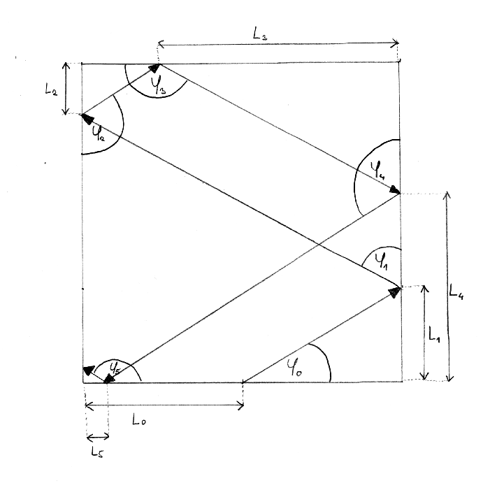
Each side is 1 unit long. The initial parameters are therefore the angle φ(0) and the distance L(0) from the left edge of the side. A ball released in this way will then bounce, yielding pairs of numbers φ(1) and L(1), then φ(2) and L(2), and so on… Therefore, if we want to prove whether the trajectory will close at a given initial angle and distance from the left edge of the side, we are interested in whether there exist numbers φ(n) and L(n) such that φ(0) = φ(n) and L(0) = L(n). In other words, we are interested in whether the ball will eventually return to the point from which it was released and bounce off it at the same angle. To better understand what happens mathematically during these bounces, I wrote an algorithm that takes two parameters—φ(n) and L(n). The algorithm then precisely calculates the values of φ(n + 1) and L(n + 1), that is, the values for the next bounce.
POKUD φ(n) < 90°:

            POKUD tan(φ(n)) * (1 – L(n)) < 1:
                        φ(n + 1) = 90° - φ(n)
                        L(n + 1) = tan(φ(n)) * (1 – L(n))

            POKUD tan(φ(n)) * (1 – L(n)) = 1:
                        φ(n + 1) = φ(n)
                        L(n + 1) = 0

            POKUD tan(φ(n)) * (1 – L(n)) > 1:
                        φ(n + 1) = 180° -  φ(n)
                        L(n + 1) = 1 – (tan(90° - φ(n)) + L(n))

POKUD φ(n) = 90°:

            φ(n + 1) = φ(n)
            L(n + 1) = L(n)

POKUD φ(n) > 90°:

            POKUD tan(180° -  φ(n)) * L(n) < 1:
                        φ(n + 1) = 270° - φ(n)
                        L(n + 1) = 1 – (tan(180° - φ(n)) * L(n))

            POKUD tan(180° -  φ(n)) * L(n) = 1:
                        φ(n + 1) = φ(n)
                        L(n + 1) = 1

            POKUD tan(180° -  φ(n)) * L(n) > 1:
                        φ(n + 1) = 180° - φ(n)
                        L(n + 1) = 1 + tan(150° - φ(n)) - L(n)
So all we need to do is feed just two basic parameters (the initial angle and position) into the algorithm, and it will give us the two parameters for the next step. We can gradually add these pairs of numbers to a set of numerical sequences (let’s call this set M). The question “Will the ball’s trajectory ever close?” is logically equivalent to the question “Is the sequence M periodic?” Unfortunately, I do not yet know how to answer this question.
I decided to continue working on the bounce simulation and extend it to 3D. In this simulation, the ball bounces off the walls of a cube in three-dimensional space. Unfortunately, this simulation cannot be used on the web as an interactive frame. Therefore, only the code and the output in the form of images are provided here.
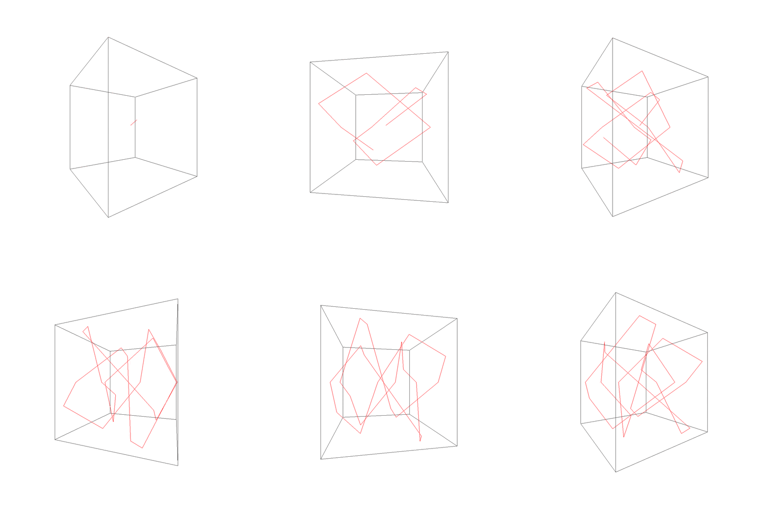
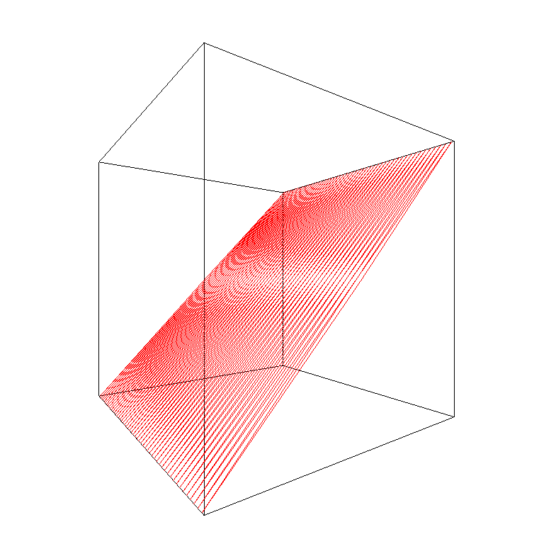
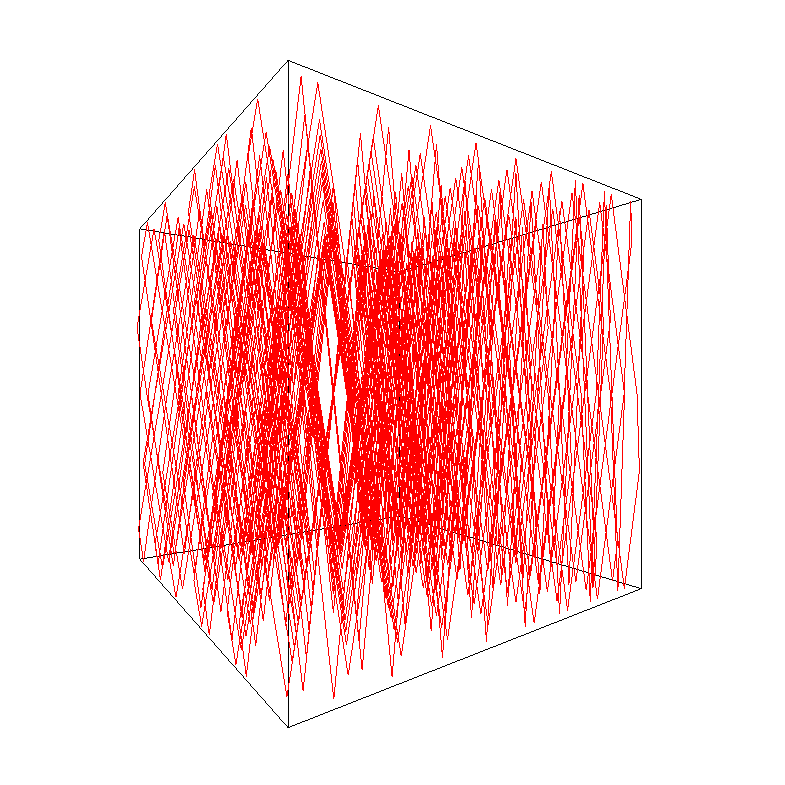
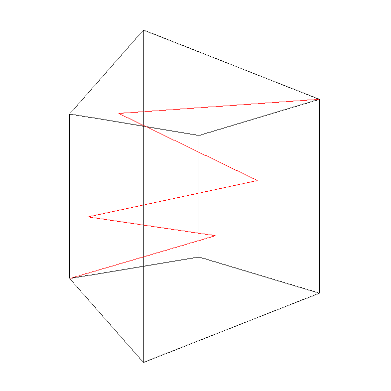
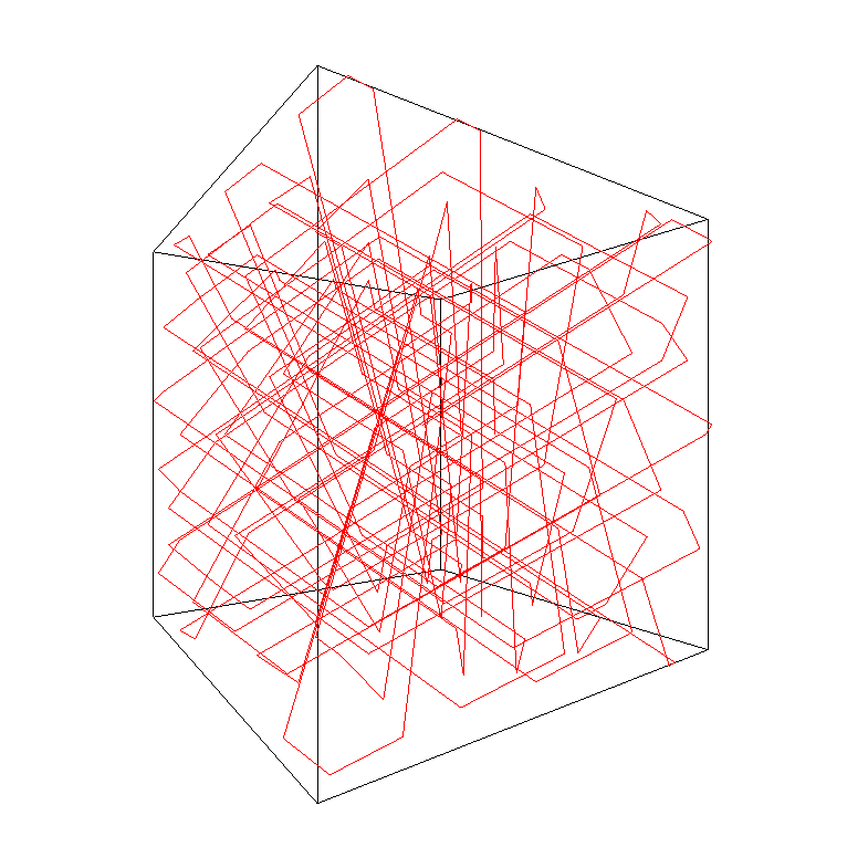
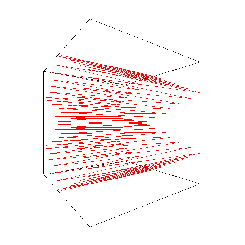
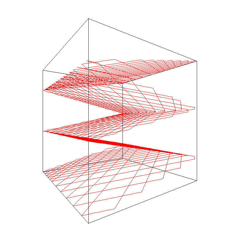
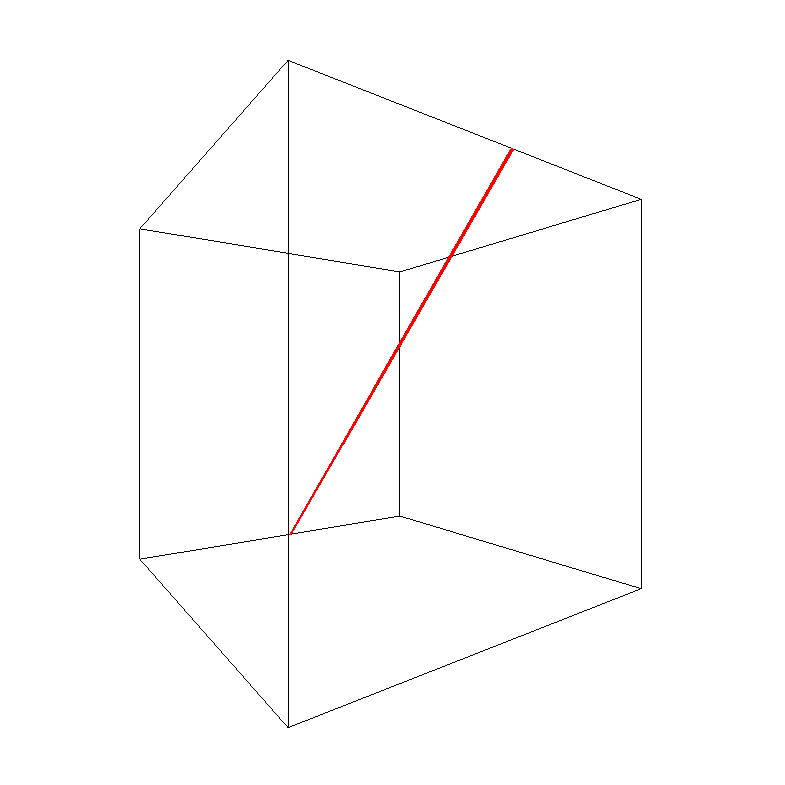
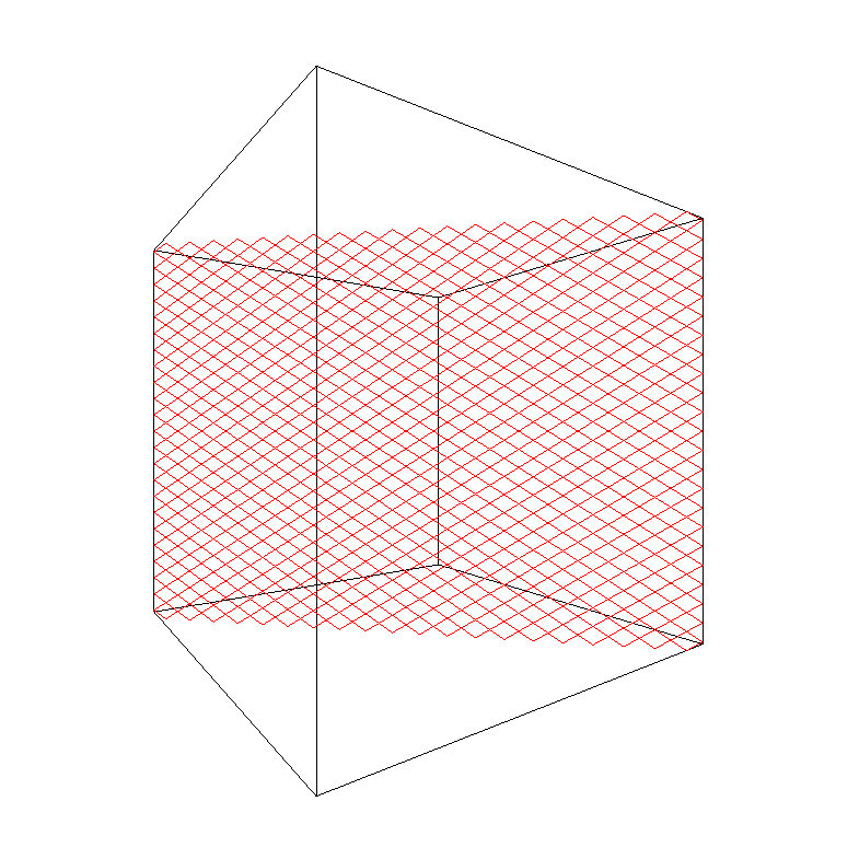
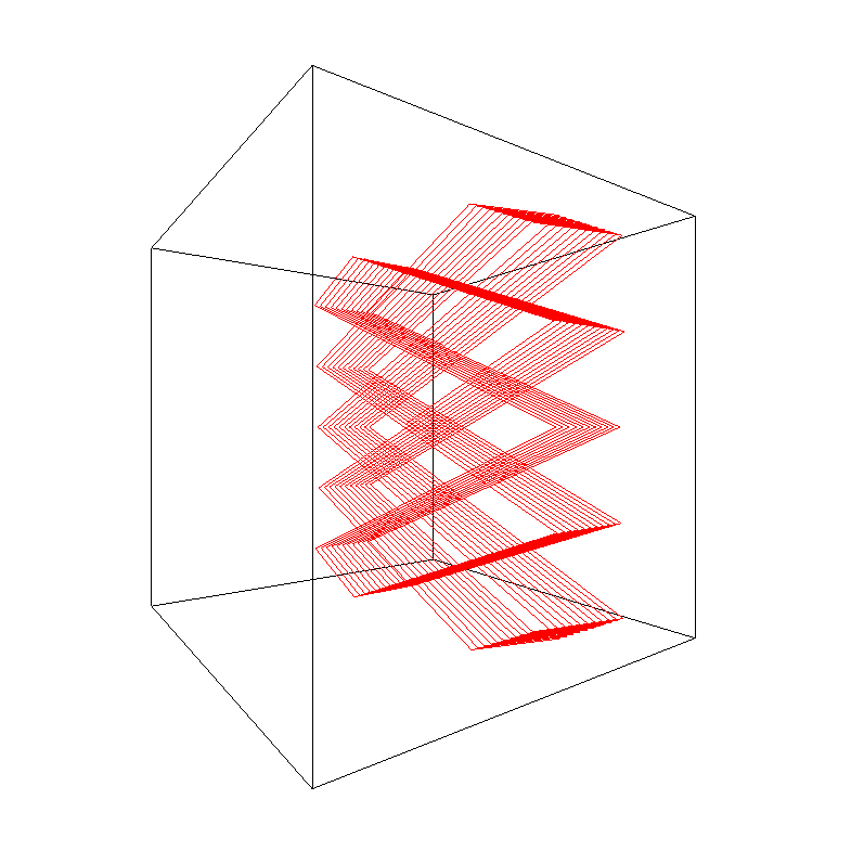
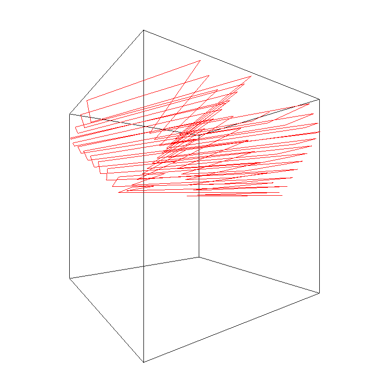
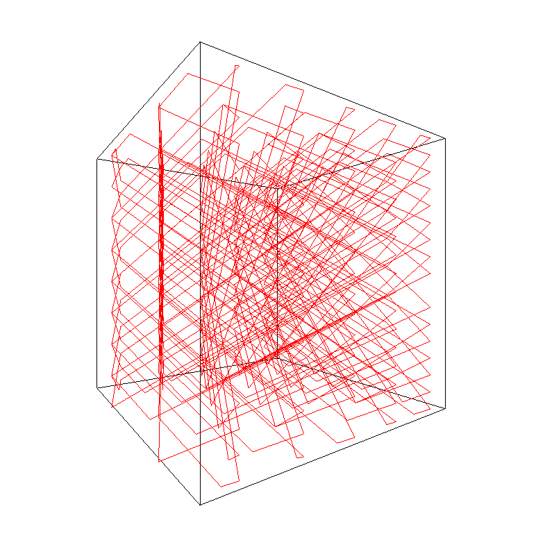
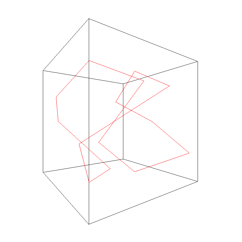
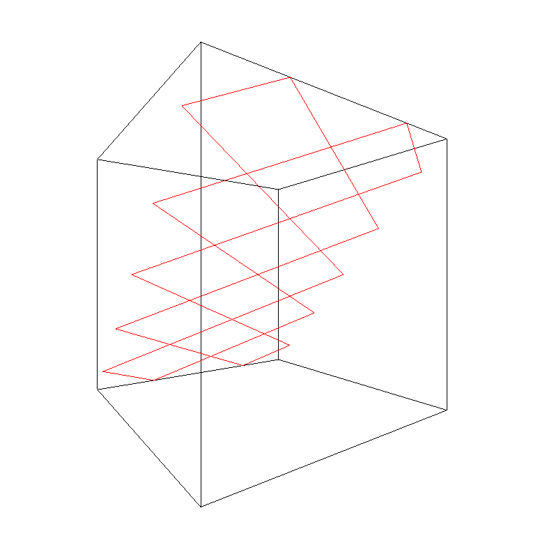
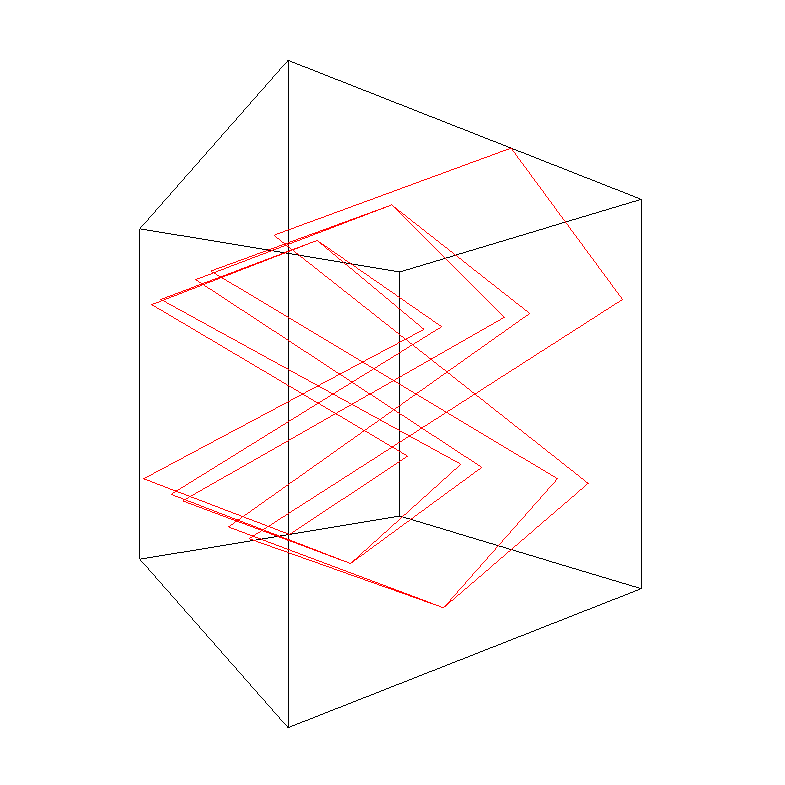
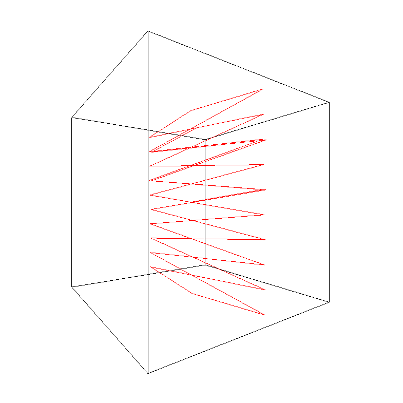
The various images above are generated by releasing the ball from the center of the cube in different directions. As you can see, this initial direction significantly affects the shape of the trajectory. Some trajectories close in on themselves after just a few bounces, while others appear rather chaotic. Just as with the 2D simulation, it is quite difficult to determine whether even very chaotic-looking trajectories will eventually close in on themselves after a sufficient number of bounces and simply trace each other from that point on. Below is an interactive demo I created for this 3D simulation.